A bright pixel is the end of a measurement chain
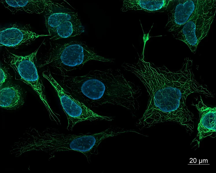
Fluorescence begins when a molecule absorbs light at a suitable wavelength and later emits some of that energy as light at a longer wavelength. A microscope selects excitation and emission bands, directs illumination onto a sample, collects a fraction of the emitted photons and converts them into detector values. The image is therefore several steps removed from a molecule count. Signal depends on how much labeled material is present, but also on how efficiently the label is excited, how much emitted light reaches the detector and how the detector records it. [1]
This chain explains why two images can look different even when the underlying biology is unchanged. A lamp may drift, an objective may collect a different fraction of light, filters may pass different wavelengths, or a camera may use another gain or exposure. In multicolor work, overlapping excitation or emission can also send some of one label into another channel. Brightness is meaningful only alongside the conditions that produced it; the color display alone cannot identify which link changed.
When concentration and fluorescence move together
In a sufficiently dilute, optically simple sample, adding more of the same fluorescent species can increase detected fluorescence in an approximately proportional way, provided illumination, geometry and detection settings stay fixed. That limited range makes a calibration series possible: measure known concentrations, fit the response over the validated interval, then compare an unknown measured under the same conditions. The proportionality is an experimental property of a setup and sample, not a universal conversion from camera value to molecule number. [2]
The relationship can bend at higher absorbance. Molecules nearer the illuminated surface absorb some of the excitation light before it reaches deeper parts of the sample; emitted photons can also be absorbed before leaving. These primary and secondary inner-filter effects make intensity rise more slowly than concentration, or otherwise distort the measured curve. The 2022 microplate study experimentally examined how optical density and well geometry affect that nonlinearity and tested a focus-position method for correction. Its result is useful evidence about microplate measurements, not a correction recipe that automatically transfers to every microscope or sample.
The label changes the biology it is meant to report
Fluorescent dyes and proteins are not invisible tags. A dye must bind, enter or be attached to a target, and labeling may vary between cells or experiments. A fluorescent protein fusion can affect the tagged protein’s localization or function; the maturation of the fluorophore and the local chemical environment can affect how much light it emits. The Nature Methods reporting guidance emphasizes identifying the exact fluorophore and its construction because variants with similar colors can differ in brightness, photostability and maturation. [1]
This creates a distinction between fluorescence and abundance. More signal could mean more target molecules, more complete labeling, a brighter molecular environment or better collection. Less signal could mean fewer targets, incomplete maturation, chemical quenching or damage from illumination. Biological controls help separate these possibilities: an unlabeled sample estimates autofluorescence, a labeling control tests specificity, and a stable reference can reveal session-to-session drift. No single control answers every question, so the control should match the proposed interpretation.
Illumination makes a signal and can erase it
Increasing excitation light often increases emitted fluorescence over a useful range, but it can also speed photobleaching: irreversible chemical changes leave fluorophores unable to emit as before. A time series can therefore appear to show a biological decline when some of the decline came from repeated imaging. A 2016 experimental comparison of fluorescent proteins measured bleaching under different illumination powers and microscopy modes; many proteins showed bleaching that rose faster than a simple linear scaling with power. The behavior depended on the fluorophore and conditions, so “twice the light means twice the damage” is not a safe general rule. [3]
A practical acquisition plan limits unnecessary exposure while keeping the signal above background and within the detector range. Focusing through the fluorescence channel can bleach the field before the recorded image; transmitted light can reduce that exposure when it is available. For comparisons across samples, keep excitation, exposure time, filters, objective, detector gain and processing consistent, and record them. The reporting guidelines also emphasize illumination stability and metadata because different instruments can produce different apparent intensities from comparable samples. [1]
A detector has a floor and a ceiling
A detector cannot distinguish every faint signal from noise, and it cannot preserve intensity differences after pixels reach their maximum recordable value. Near the low end, background and photon-counting fluctuations make estimates uncertain. At the high end, saturation clips distinctions: two areas with different underlying brightness may both be recorded at the same maximum value. Contrast stretching in display software can make a dim image look vivid, but it changes appearance rather than recovering missing measurements. Quantitative analysis should use raw or minimally processed data and check the intensity histogram for saturated pixels.
Background subtraction is also a model choice. A nearby empty region can estimate local background, but it may not represent background inside a cell or tissue, where autofluorescence and scattering vary. The microscopy guidance recommends validating performance and reporting acquisition details; flat-field correction can address uneven illumination when a suitable reference is measured, but an inaccurate reference can add error. [1] A careful workflow records how regions were selected, how background was estimated and whether correction was applied before interpreting a mean intensity.
A worked example shows what a ratio can support
Imagine two groups of cells labeled with the same fluorescent probe. With identical imaging settings, the measured average signals are 120 and 150 arbitrary units. The raw ratio is 150/120 = 1.25, a 25% higher measured signal in the second group. This is an arithmetic example, not experimental data. It supports the narrow statement that the measured fluorescence was higher under the stated acquisition and analysis conditions. It does not alone establish 25% more target molecules.
To support an abundance interpretation, the comparison would need evidence that labeling efficiency, cell size or sampled volume, background, illumination, detector range and fluorophore environment are comparable, or a validated normalization that accounts for differences. If the values came from separate days, a fluorescent reference standard could help assess instrument drift. If one group approached saturation, the ratio would be unreliable. The experimental question determines whether mean intensity, integrated signal per cell, a fluorescence ratio or another measure is the relevant quantity.
Ratios and calibration solve different problems
A ratiometric probe measures two optical signals whose ratio changes with a condition such as pH or ion binding. Some shared variation in probe amount or illumination can cancel in the ratio, but only when the probe’s response and measurement channels behave as assumed. The historical pH ratio-imaging work demonstrated calibration and controls for its particular probe and cellular setup; that does not make every two-color ratio immune to focus, bleed-through, background or saturation. [1]
A calibration curve instead maps signal to known standards under specified conditions. It can estimate a concentration inside the validated range, but changes in sample matrix or optical path can break the mapping. The recent microplate study underscores that concentration linearity is limited by optical density and geometry. [2] Thus, normalization, ratiometry and calibration are different tools: each addresses particular sources of variation and each needs validation for the actual sample and instrument.
Make the claim match the measurement
A reader should be able to tell what made the sample fluorescent, which excitation and emission settings were used, what microscope and detector collected the signal, and how images were processed. For a quantitative comparison, report the acquisition settings, controls, sampling plan, background method and analysis measure. Include enough information to judge whether images were collected within the detector’s dynamic range and whether illumination or bleaching could have changed the signal. These details are not decoration; they define what an intensity comparison means. [1]
Fluorescence remains a powerful way to locate molecules, follow processes and compare samples. Its strength comes from converting otherwise difficult-to-see molecular behavior into measurable light. The same conversion brings optical, chemical and instrumental assumptions into the result. Treating brightness as a measurement with boundaries—rather than a transparent count—lets the image guide a sound question without asking it to prove more than the experiment established.
Fluorescence intensity is a measured light signal, not a direct count of molecules. A defensible comparison controls the label and imaging conditions, checks background and detector range, and reports how the signal was acquired and analyzed.
Sources & further reading
Numbered references connect claims to their source. The main text is our original explanation; conceptual examples are identified as imagined.
- Montero Llopis et al. — Best practices and tools for reporting reproducible fluorescence microscopy methodsMethods perspective · Nature Methods · 7 June 2021
- Friganović et al. — Inner Filter Effect Correction for Fluorescence Measurements in Microplates Using Variable Vertical Axis FocusPrimary analytical chemistry study · Analytical Chemistry · 2022
- Cranfill et al. — Quantitative Assessment of Fluorescent ProteinsPrimary study · Nature Methods · 30 May 2016
Source review: 16 Nov 2026. Editorial standards.